Motor Selection
1b) Motor Selection
SG90 Specification
●	Rotation : 0°-180°


●	Weight of motor : 9gm


●	Operating Voltage : +5 V


●	Stall Current : 350 mA


●	Stall Torque : 2.5 kg . cm = 0.24 N.m


●	Speed : 0.12s / 60° = 82.8 rpm


●	Power : Torque * Speed / 9.5488 = 2.08 kW
This motor was selected due to the requirement of having a very lightweight actuator which did not lack the torque to move the entire load of the robot.
Power Supply Selection
1c) Power Supply Selection:
Given the stall current of the motors being used, a power supply capable of supplying far more than 350 mA is required. An Alkaline 9v battery is chosen as the power supply for the system which satisfies this requirement and has enough battery capacity to sustain the robot to operate for a reasonable span of time.
Static Friction Calculation
Static Friction Calculation:
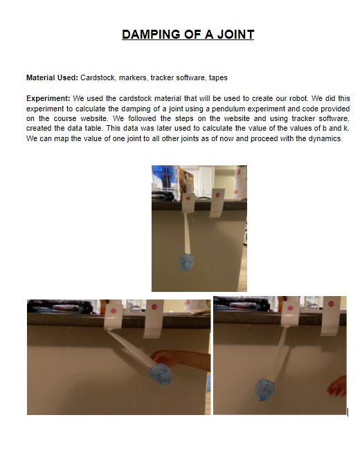
The Angle of Repose experiment was conducted to determine the static friction coefficient of the cardstock on a smooth surface. The platform having the cardstock is lifted slowly with increasing angle to find that critical angle at which the paper starts sliding down.
Trial 1:
Coefficient of Static Friction : 0.3141
Trial 2 :
Coefficient of Static Friction : 0.4575
Trial 3 :
Coefficient of Static Friction : 0.3803
Average Coefficient of Static Friction : 0.38399
Average Coefficient of Static Friction : 0.3057
Approximation : The coefficient of kinetic friction could be determined during the same Angle of Repose experiment where the angle corresponding to when the cardstock slips down the inclined surface at constant velocity is noted. An angle of ~17 degrees let the cardstock slip down in an approximately constant velocity. Thus coefficient of kinetic friction = tan (17) = 0.3057
Compliance Calculation Using Two-Beam Method
import sympy
q = sympy.Symbol('q')
d = sympy.Symbol('d')
L = sympy.Symbol('L')
P = sympy.Symbol('P')
h = sympy.Symbol('h')
b = sympy.Symbol('b')
E = sympy.Symbol('E')
x = sympy.Symbol('x')
subs = {}
#subs[k]=1000
subs[P]=.0098
subs[L]=.100
subs[b]=.025
subs[h]=.005
subs[E]= 1.551e9
subs[x]=.5
I = b*h**3/12
d1 = P*L**3/3/E/I
d1.subs(subs)
$\displaystyle 8.08768536428111 \cdot 10^{-6}$
q1 = P*L**2/2/E/I
q1.subs(subs)
$\displaystyle 0.000121315280464217$
k1 = P*L*(1-x)/(sympy.asin(P*L**2/(3*E*I*(1-x))))
k1.subs(subs)
$\displaystyle 3.02929686179011$
d2 = L*(1-x)*sympy.sin(P*L*(1-x)/k1)
d2.subs(subs)
$\displaystyle 8.08768536428111 \cdot 10^{-6}$
q2 = P*L*(1-x)/k1
q2.subs(subs)
$\displaystyle 0.000161753707990983$
k2 = 2*E*I*(1-x)/(L)
k2
$\displaystyle \frac{E b h^{3} \left(1 - x\right)}{6 L}$
q3 = P*L*(1-x)/k2
q3.subs(subs)
$\displaystyle 0.000121315280464217$
d3 = L*(1-x)*sympy.sin(P*L*(1-x)/k2)
d1.subs(subs)
$\displaystyle 8.08768536428111 \cdot 10^{-6}$
d3.subs(subs)
$\displaystyle 6.06576400833212 \cdot 10^{-6}$
del subs[x]
error = []
error.append(d1-d2)
error.append(q1-q2)
error= sympy.Matrix(error)
error = error.subs(subs)
error
$\displaystyle \left[\begin{matrix}0\0.000121315280464217 - \operatorname{asin}{\left(\frac{8.08768536428111 \cdot 10^{-5}}{1 - x} \right)}\end{matrix}\right]$
import scipy.optimize
f = sympy.lambdify((x),error)
def f2(args):
    a = f(*args)
    b = (a**2).sum()
    return b
sol = scipy.optimize.minimize(f2,[.25])
sol
      fun: 1.816962570090524e-10
 hess_inv: array([[1]])
      jac: array([-3.87618667e-09])
  message: 'Optimization terminated successfully.'
     nfev: 2
      nit: 0
     njev: 1
   status: 0
  success: True
        x: array([0.25])
subs[x]=sol.x[0]
d2.subs(subs)
$\displaystyle 8.08768536428111 \cdot 10^{-6}$
q2.subs(subs)
$\displaystyle 0.000107835805066077$
k2.subs(subs)
$\displaystyle 6.05859375$
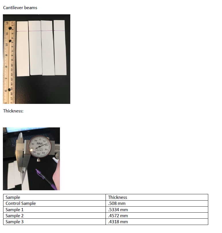
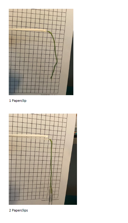
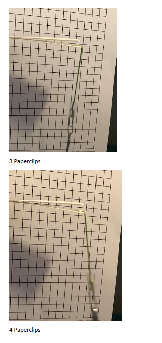
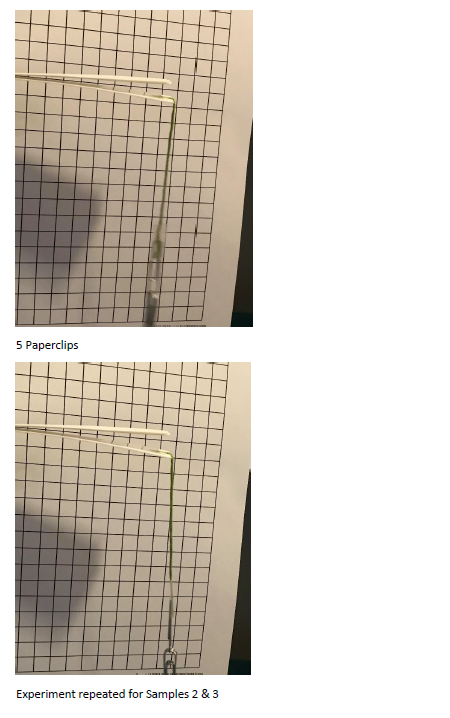
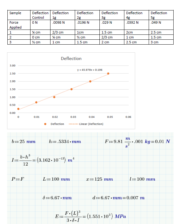
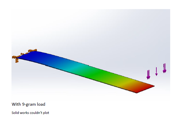
Cantilever Beams Material Experiment
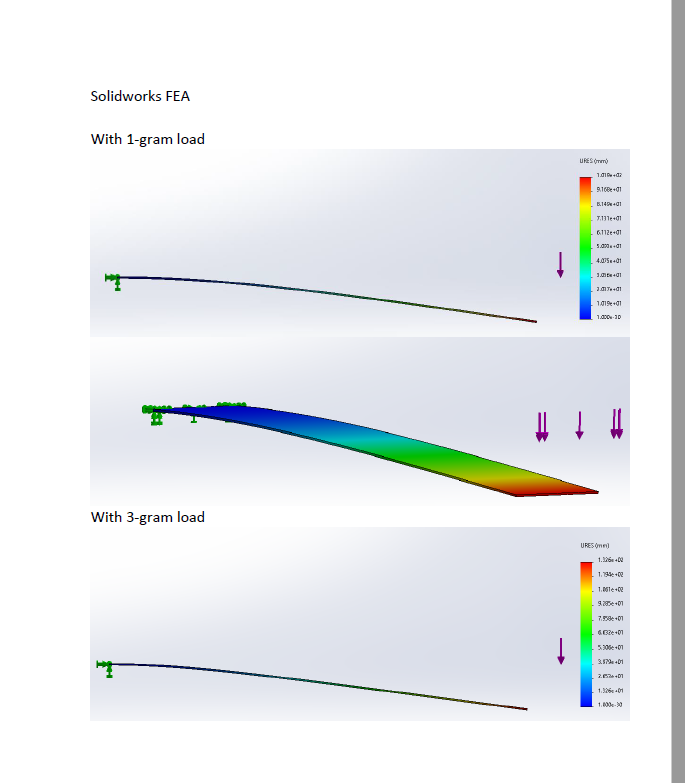
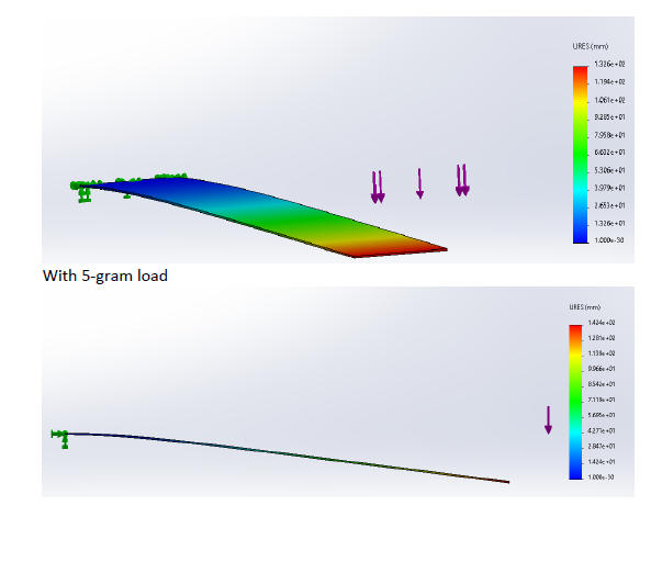
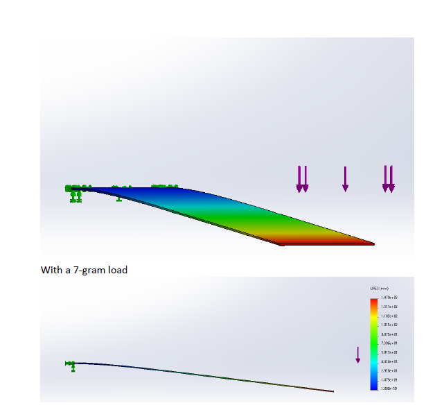
Solidworks Bending FEA
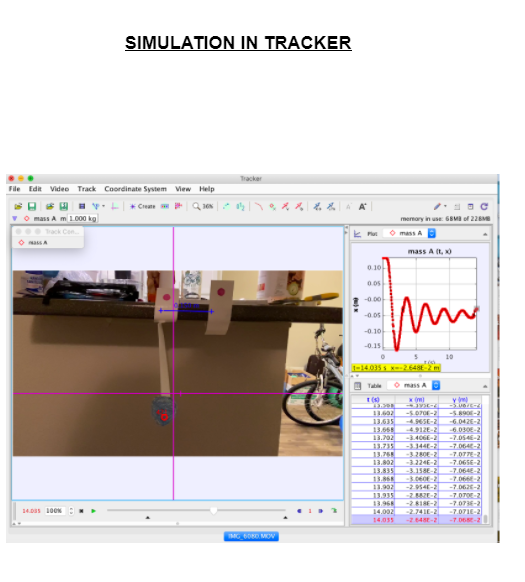
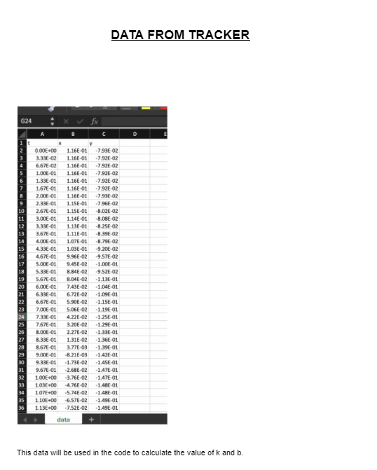
Joint Damping Data Collection
Joint Damping Calculations
import pynamics
from pynamics.frame import Frame
from pynamics.variable_types import Differentiable,Constant
from pynamics.system import System
from pynamics.body import Body
from pynamics.dyadic import Dyadic
from pynamics.output import Output,PointsOutput
from pynamics.particle import Particle
import pynamics.integration
import numpy
import matplotlib.pyplot as plt
plt.ion()
from math import pi

import logging
import pynamics.integration
import pynamics.system
import numpy.random
import scipy.interpolate
import scipy.optimize
#import cma
import pandas as pd
import numpy
import matplotlib.pyplot as plt
import scipy.interpolate as si
system = System()
pynamics.set_system(__name__,system)

lA = Constant(1,'lA',system)
lB = Constant(1,'lB',system)
lC = Constant(1,'lC',system)

mA = Constant(1,'mA',system)
mB = Constant(1,'mB',system)
mC = Constant(1,'mC',system)

g = Constant(9.81,'g',system)
b = Constant(1e1,'b',system)
k = Constant(1e1,'k',system)

preload1 = Constant(0*pi/180,'preload1',system)
preload2 = Constant(0*pi/180,'preload2',system)
preload3 = Constant(0*pi/180,'preload3',system)

Ixx_A = Constant(1,'Ixx_A',system)
Iyy_A = Constant(1,'Iyy_A',system)
Izz_A = Constant(1,'Izz_A',system)
Ixx_B = Constant(1,'Ixx_B',system)
Iyy_B = Constant(1,'Iyy_B',system)
Izz_B = Constant(1,'Izz_B',system)
Ixx_C = Constant(1,'Ixx_C',system)
Iyy_C = Constant(1,'Iyy_C',system)
Izz_C = Constant(1,'Izz_C',system)

tol = 1e-12

tinitial = 0
tfinal = 10
fps = 30
tstep = 1/fps
t = numpy.r_[tinitial:tfinal:tstep]

qA,qA_d,qA_dd = Differentiable('qA',system)
qB,qB_d,qB_dd = Differentiable('qB',system)
qC,qC_d,qC_dd = Differentiable('qC',system)

initialvalues = {}
initialvalues[qA]=-45*pi/180
initialvalues[qA_d]=0*pi/180
initialvalues[qB]=0*pi/180
initialvalues[qB_d]=0*pi/180
initialvalues[qC]=0*pi/180
initialvalues[qC_d]=0*pi/180

statevariables = system.get_state_variables()
ini = [initialvalues[item] for item in statevariables]

N = Frame('N')
A = Frame('A')
B = Frame('B')
C = Frame('C')

system.set_newtonian(N)

A.rotate_fixed_axis_directed(N,[0,0,1],qA,system)
B.rotate_fixed_axis_directed(A,[0,0,1],qB,system)
C.rotate_fixed_axis_directed(B,[0,0,1],qC,system)

pNA=0*N.x
pAB=pNA+lA*A.x
pBC = pAB + lB*B.x
pCtip = pBC + lC*C.x

pAcm=pNA+lA/2*A.x
pBcm=pAB+lB/2*B.x
pCcm=pBC+lC/2*C.x

wNA = N.getw_(A)
wAB = A.getw_(B)
wBC = B.getw_(C)

IA = Dyadic.build(A,Ixx_A,Iyy_A,Izz_A)
IB = Dyadic.build(B,Ixx_B,Iyy_B,Izz_B)
IC = Dyadic.build(C,Ixx_C,Iyy_C,Izz_C)

BodyA = Body('BodyA',A,pAcm,mA,IA,system)
BodyB = Body('BodyB',B,pBcm,mB,IB,system)
BodyC = Body('BodyC',C,pCcm,mC,IC,system)

system.addforce(-b*wNA,wNA)
system.addforce(-b*wAB,wAB)
system.addforce(-b*wBC,wBC)

system.add_spring_force1(k,(qA-preload1)*N.z,wNA)
system.add_spring_force1(k,(qB-preload2)*N.z,wAB)
system.add_spring_force1(k,(qC-preload3)*N.z,wBC)

system.addforcegravity(-g*N.y)
eq = []
# eq.append(pCtip.dot(N.y))
eq_d=[(system.derivative(item)) for item in eq]
eq_dd=[(system.derivative(item)) for item in eq_d]

f,ma = system.getdynamics()
2021-03-19 23:04:28,290 - pynamics.system - INFO - getting dynamic equations
unknown_constants = [b,k]
known_constants = list(set(system.constant_values.keys())-set(unknown_constants))
known_constants = dict([(key,system.constant_values[key]) for key in known_constants])
func1,lambda1 = system.state_space_post_invert(f,ma,eq_dd,return_lambda = True,constants = known_constants)
2021-03-19 23:04:28,464 - pynamics.system - INFO - solving a = f/m and creating function
2021-03-19 23:04:28,749 - pynamics.system - INFO - substituting constrained in Ma-f.
2021-03-19 23:04:28,868 - pynamics.system - INFO - done solving a = f/m and creating function
2021-03-19 23:04:28,869 - pynamics.system - INFO - calculating function for lambdas
def run_sim(args):
    constants = dict([(key,value) for key,value in zip(unknown_constants,args)])
    states=pynamics.integration.integrate(func1,ini,t,rtol=tol,atol=tol,hmin=tol, args=({'constants':constants},))
    return states
points = [pNA,pAB,pBC,pCtip]
#create data
points_output = PointsOutput(points,system)
df=pd.read_csv(r'/Users/sanchit/Downloads/data.csv', sep=',')
x = df.x.to_numpy()
y = df.y.to_numpy()
t = df.t.to_numpy()
xy = numpy.array([x,y]).T
fy = scipy.interpolate.interp1d(t,xy.T,fill_value='extrapolate')
fyt = fy(t).T
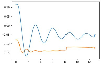
plt.figure()
plt.plot(t,fyt)
[<matplotlib.lines.Line2D at 0x7f959296e450>,
 <matplotlib.lines.Line2D at 0x7f959296e650>]
def calc_error(args):
    states_guess = run_sim(args)
    y_guess = points_output.calc(states_guess)
    y_guess = y_guess.reshape((390,-1))
    print(y_guess.shape)
    error = fyt - y_guess
    error **=2
    error = error.sum()
    return error
pynamics.system.logger.setLevel(logging.ERROR)
k_guess = [1e2,1e3]
method = None
#method = 'CMA'
#method = 'BFGS'

if method is None:
    result = k_guess
elif method == 'CMA':
    es = cma.CMAEvolutionStrategy(k_guess, 0.5)
    es.logger.disp_header()
    while not es.stop():
          X = es.ask()
          es.tell(X, [calc_error(x) for x in X])
          es.logger.add()
          es.logger.disp([-1])
    result = es.best.x
else:
    sol = scipy.optimize.minimize(calc_error,k_guess,method = method)
    print(sol.fun)
    result = sol.x
calc_error(result)
2021-03-19 23:04:29,110 - pynamics.integration - INFO - beginning integration
2021-03-19 23:04:33,853 - pynamics.integration - INFO - finished integration
2021-03-19 23:04:33,854 - pynamics.output - INFO - calculating outputs
2021-03-19 23:04:33,922 - pynamics.output - INFO - done calculating outputs


(390, 8)


---------------------------------------------------------------------------

ValueError                                Traceback (most recent call last)

<ipython-input-14-9e227d5729d7> in <module>
----> 1 calc_error(result)


<ipython-input-10-4e201c5927ca> in calc_error(args)
      4     y_guess = y_guess.reshape((390,-1))
      5     print(y_guess.shape)
----> 6     error = fyt - y_guess
      7     error **=2
      8     error = error.sum()


ValueError: operands could not be broadcast together with shapes (390,2) (390,8)
calc_error(k_guess)